Use and remove stationarity?

‘If we fit a stationary model to data, we assume our data are a realization of a stationary process. So our first step in an analysis should be to check whether there is any evidence of a trend or seasonal effects and, if there is, remove them.’ —Introductory Time Series with R.

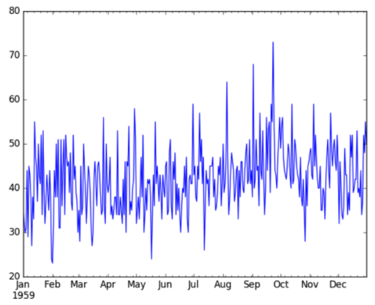
A time series is stationary, that means the statistical properties such as mean, variance, autocorrelation are all consistent over time. Stationary time series can be easier to model. Let’s see a example of stationary data:

On contrast, non-stationary dataset shows seasonality, cycles and other structures that depend on the time index. Summary statistics such as mean and variance change over time, and make the model hard to capture the important factor. Like previous posts where we talked about detrend and correct seasonal factors, classical time series analysis and forecasting methods concerned with making non-stationary data to stationary data. Let’s see an example of non-stationary data:

By looking at plots above, we know there is a seasonal trend in our dataset, and therefore, the data is non-stationary. There are also other ways to check for stationary, such as summary statistics and statistical tests.

Summary Statistics:#

Checking summary statistics is one of the ways to see if a time series is stationary or non-stationary. If a time series is stationary, the mean and variance should be consistent over time. We can then split our dataset into different groups and calculates the mean and variance of each group. Let us use the previous sales data as an example:

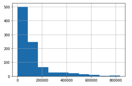
data2.hist()

By looking at the histogram, we know that the data is highly right skewed. Next, we will split the data into two groups and calculates the mean and variance of each group.

length=len(data2)/2
split=int(length)
X1=data2[0:split]
X2=data2[split:]
mean1=X1.mean()
mean2=X2.mean()
var1=X1.var()
var2=X2.var()
print('mean1:', mean1, "mean2:", mean2)
print('var1:', var1, 'var2:', var2)

Output: 
mean1: 72517.85470459521 mean2: 152722.51681222717
var1: 9433357685.309347 var2: 23493684358.79559

By looking at the mean and variance from two groups, we can definitely say that the time series is non-stationary. Also, by looking at the plot again, it looks like that the seasonality is growing, and suggests an exponential growth from season to season. Therefore, we can use log transformation to flatten out the exponential factor. As the line plot shown below, the exponential growth seems to be diminished compared to previous plot.

X=data2.values
X=np.log(X)
f=plt.figure()
f.set_figwidth(15)
pyplot.plot(X)

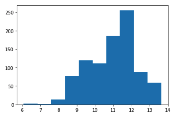
pyplot.hist(X)

Running the code above plot the histogram. We can see that the histogram is more like a Gaussian distribution, rather than right skewed. Now, let’s calculates the mean and variance across the groups after the log transformation:

split2=int(len(X)/2)
X3, X4=X[0:split], X[split:]
mean3, mean4=X3.mean(), X4.mean()
var3, var4=X3.var(), X4.var()
print("mean3:", mean3, "mean4:", mean4)
print("var3:", var3, "var4:", var4)

[output]
mean3: 10.480743900555884 mean4: 11.429529392014638
var3: 1.5453799930195664 var4: 1.2788258644987915

Running the code above shows the mean and variance that are very close to each other. This means that we transformed our non-stationary dataset to stationary.

Augmented Dickey-Fuller test#

The Augmented Dickey-Fuller test is also called a unit root test. The intuition behind is to determine how strongly a time series is defined by a trend. The null hypothesis of the test is that the time series can be represented by a unit root, that it is not stationary, it has time dependent structures. The alternative hypothesis is that the time series is stationary. If p-value is below a threshold (for example 5%), then we reject the null hypothesis, and thus the time series is stationary. Otherwise, we fail to reject the null hypothesis that means the time series is non-stationary.

from statsmodels.tsa.stattools import adfuller
X_augmented=data2.values
result=adfuller(X_augmented)
print('ADF statistics: ', result[0])
print('p-value:' ,result[1])
print('key value:')
for key, value in result[4].items():
    print((key, value))

[output]
ADF statistics:  -4.253573724998073
p-value: 0.0005340353910033514
key value:
('1%', -3.437694005510983)
('5%', -2.8647819837978683)
('10%', -2.5684962548451375)

Running the code suggests that we can reject the null hypothesis, and thus our dataset is stationary or does not have time-dependent structure.

Conclusion:#

There are couple methods to check if a time series is stationary or non-stationary. Most easy one is to plot and see the basic summary such as mean and variance. We can also calculate the p-value to check if the time series is stationary or not.