Use and remove trends in time series analysis?

Trend is one of the characteristics of time series data. In this article, we will talk about trends and how to remove them.

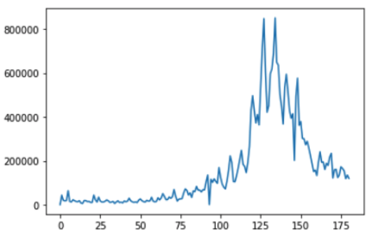
Trend is a continued increase or decrease in the series over time. There are different types of trends, such as deterministic trend, which are trends that are consistently increasing or decreasing. Another trend type that changes inconsistently(stochastic trends). Identifying trends in time series datasets can lead to faster modeling, simplification of the problems and improvement upon model performance. There are different ways to identify a trend, but the most common way is to plot it and visualize the dataset. Here is an example:

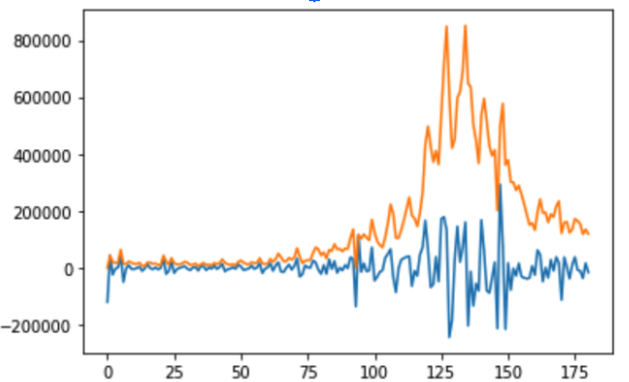
Detrend by Differencing: The simplest method to detrend a time series is by differencing – calculating the current time steps as the difference between original observations and previous time steps. Let’s see an example of detrending previous example:

X=data1.values
diff=list()
for i in range(0, len(X)):
    Z=X[i]-X[i-1]
    diff.append(Z)
diff
from matplotlib import pyplot
# Compare before and after remove trend:
pyplot.plot(diff)
pyplot.plot(X)

Running the previous example creates the new detrended dataset (plotted in blue). By comparing the original plot(orange line), the trend does appear to have been removed.

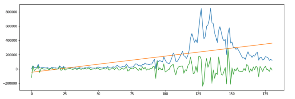
Detrending by Model Fitting: A trending is often easily visualized as a line through the observations. By subtracting prediction values from the observation values, the residuals can be used to detrend a time series.

Value(t)=observation(t)-prediction(t)

By doing this, the residuals of the fit of the model will be used as a detrended form. Therefore, we need to fit our data with linear regression model first, and then subtract it from the original dataset. Let’s see an example:

from sklearn.linear_model import LinearRegression

X2=[i for i in range(0, len(data1))]
X2=np.reshape(X2, (len(X2), 1))
y1=data1.values

linear_model=LinearRegression()
linear_model.fit(X2, y1)
y3=linear_model.predict(X2)

f = plt.figure()
f.set_figwidth(15)
f.set_figheight(5)
plt.plot(y1)
plt.plot(y3)
pyplot.plot(diff)

The orange line shows the trend after detrending with linear regression, where the green line is used to represent the detrend. We can see the difference clearly where detrending by model fitting is more effective compared to differencing method.

Conclusion:#

In this article, we talked about detrending time series dataset. It shows two methods to remove the trend – by subtracting the previous time step values and by fitting a linear model. The example concludes that using the model fitting method is more effective in terms of detrending a time series data. The future post will explore more techniques in time series analysis.

Reference:#

Introduction to Time Series Forecasting with Python: How to Prepare Data and Develop Models to Predict the Future (Jason Brownlee)