Use and remove seasonality in time series analysis?

“A repeating pattern within each year is known as seasonal variation, although the term is applied more generally to repeating patterns within any fixed period” – Introductory Time Series with R

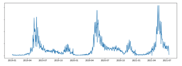
As the definition shown above, seasonality is another characteristic of time series datasets. It usually contains cycles that repeat over a specific time period. However, the repeating cycles may obscure the signal that we wish to model when conducting time series forecasting. This article will talk about how to adjust seasonality in time series data, and model the seasonal components. The most simple approach to identify seasonality is through plotting. Seasonality includes but not limited to: Time of day Daily/weekly/monthly/yearly…

f = plt.figure()
f.set_figwidth(15)
f.set_figheight(5)
plt.plot(data2)
plt.show()

Deseasonalizing (or Seasonal Adjustment):#

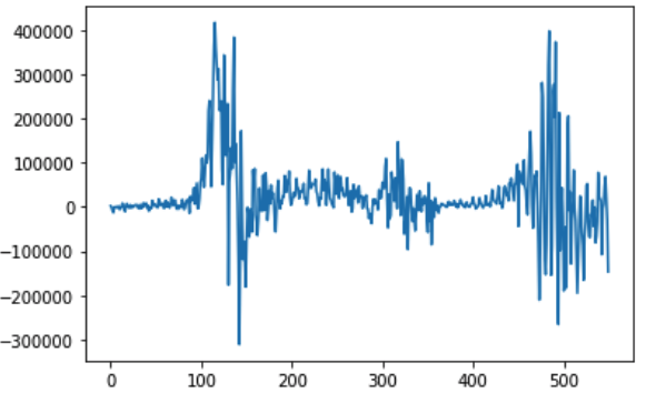
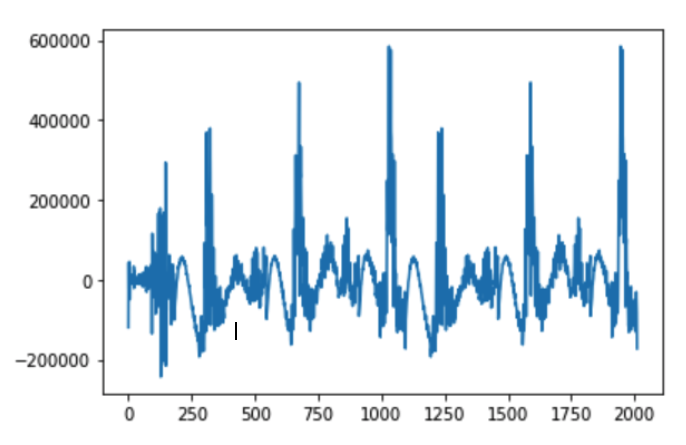
Like detrend, differencing can correct seasonal components by subtracting the value from previous time steps. In my example where the sales data shows a yearly seasonality, I will subtract the current value from the same day last year for correction. The line plot below shows the deseasonalized sales data using differencing method:

Z=data2.values
diff2=list()
days_in_year=365
for i in range(days_in_year, len(Z)):
    my_value=Z[i]-Z[i-days_in_year]
    diff2.append(my_value)
pyplot.plot(diff)

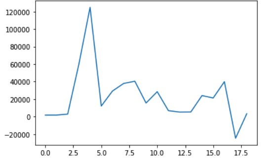
In case it come across with leap year, we can update the code or consider that consider the sales within a given period of the year is probably stable, perhaps over a few weeks. We can shortcut and consider all temperatures within a calendar month to be stable. By subtracting the average cost from the same calendar month in the previous year, we can deseason the dataset. Here comes an example:

resample_month=data2.resample('M')
monthly_mean=resample_month.mean()
#monthly_mean.plot()
diff2=list()
month_in_year=12
for i in range(month_in_year, len(monthly_mean)):
    my_values2=monthly_mean[i]-monthly_mean[i - month_in_year]
    diff2.append(my_values2)
pyplot.plot(diff2)

Seasonal Adjustment with Modeling#

We can also model the seasonal component directly and then subtract it from the observations. The seasonal component in a given time series is likely a sine wave over a generally fixed period of roughly equal amplitude. By using the polyfit() function in NumPy, we can fit a polynomial of a chosen order to our dataset. In our dataset, the time index would be the day of the year. In the example, I picked 5th order polynomial for the model.

from numpy import polyfit
C2=[i%365 for i in range(0, len(data2))]
y3=data2.values
degree=5	
coef=polyfit(C2, y3, degree)
print('coeffecient:%s' % coef)

curve=list()
for i in range(len(data2)):
    value=coef[-1]
    for d in range(degree):
        value+=C2[i]**(degree-d)*coef[d]
    curve.append(value)
pyplot.plot(data2.values)
pyplot.plot(curve, color='red', linewidth=4)

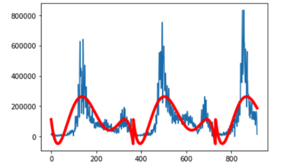
By running our model, it plots the resulting seasonal model over the top of the original dataset. The curve seems a good fit for the seasonal structure in the dataset. Then we can subtract the seasonal values from the original values to create the seasonal adjusted dataset:

values=data2.values
diff4=list()
for i in range(len(data2)):
    value=values[i]-curve[i]
    diff.append(value)
pyplot.plot(diff)

To conclude, understanding the seasonal component in time series can improve the performance of modeling. It creates a clear signal between input and output and provides new information to improve model performance.

Reference:#

Introduction to Time Series Forecasting with Python: How to Prepare Data and Develop Models to Predict the Future (Jason Brownlee)