heart disease prediction

Introduction#
Coronary heart disease (CHD) is one of the most common types of heart disease in America. Making early prognosis can help high risk potential patients to change lifesyle and reduce the chance of getting it. The objective of the project is to determine the risk factors for predicting the probability of developing CHD.
The ‘framingham’ dataset provides information whether the participants developed Coronary Heart Disease (CHD) after ten years of the study.
Data#
Now let’s import the data. The dataset includes 4,240 samples with a total of 16 columns, consisting of eight categorical and eight numerical attributes.
data=pd.read_csv("framingham.csv")
data.isnull().sum()
male 0
age 0
education 105
currentSmoker 0
cigsPerDay 29
BPMeds 53
prevalentStroke 0
prevalentHyp 0
diabetes 0
totChol 50
sysBP 0
diaBP 0
BMI 19
heartRate 1
glucose 388
TenYearCHD 0
Replace missing value with most frequent value - Education Column#
Among the seven features with missing values, there are two categorical features: education and BPMeds. Missing values of these two categorical features are replaced by “the most frequent values” within each column. Take the education column as an example:
# find the most frequent value
data['education'].value_counts()
| missing | value_counts |
|---|---|
| 1.0 | 1720 |
| 2.0 | 1253 |
| 3.0 | 689 |
| 4.0 | 473 |
#replace missing values with "1.0"
def replace_most_common(x):
	if pd.isnull(x):
		return 1.0
	else:
		return x
data['education'] = data['education'].map(replace_most_common)
Replace missing values with median - cigsPerDay#
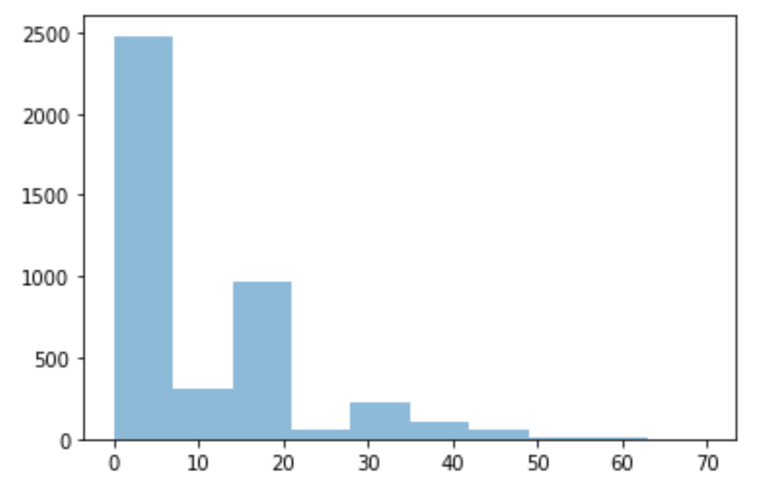
For the five numerical features (cigsPerDay, totChol, BMI, glucose, HeartRate), the missing values are replaced with the median value since due to asymmetrical distributions in the histograms. Take cigsPerDay as an example:
plt.hist(data['cigsPerDay'], alpha=0.5)

data["cigsPerDay"].fillna(data['cigsPerDay'].median(),inplace=True)
Feature Engineering - Backward elimination (p-value)#
Feature selection technique is often used in Machine Learning as a strategy to include variables from a dataset. The fundamental idea of feature selection is to fit the features that are statistically most relevant to the model.
Backward elimination is decided on a significant level for a variable to be retained in the model using a p-value. First, a model is fitted with all independent variables. Then the variable with the highest p-values is removed before the model is fitted again with the removed variable. The process continues until no further steps are necessary.
Before we begin with Backward elimination, we need to append ‘1’ at the beginning of our data set. Now, why is this important? For performing Backward elimination, we are required to use the linear model provided by statsmodels library — which does not consider the bias term. Hence, by adding a dummy feature with value as ‘1’, our equation becomes y=b.x0+m1.x1+m2.x2+m3.x3+m4.x4 where x0 = 1.
X.shape
[output]: (4240,15)
Append column of ones:
#append column of ones
X_with_ones= np.append (arr=np.ones([X.shape[0],1]).astype(int), values = X, axis = 1)
print("before Elimination, there are",X_with_ones.shape[1],"columns")

[output]:before Elimination, there are 16 columns
import statsmodels.api as sm
def backwardElimination(x, sl):
	numVars= len(x[0])
	for i in range(0, numVars):
		obj_OLS= sm.OLS(y, x).fit()
		maxVar= max(obj_OLS.pvalues).astype(float) if maxVar> sl:
			for j in range(0, numVars-i):
				if (obj_OLS.pvalues[j].astype(float) == maxVar):
					x = np.delete(x, j, 1)
	obj_OLS.summary()
	return x
SL=0.05
X_modeled=backwardElimination(X_with_ones, SL)
X_modeled.shape
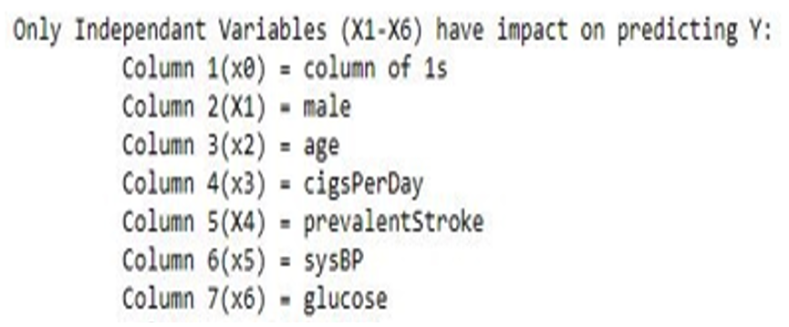
print("after backward elimination, there are 7 columns left.")

Logistic Regression:#
After splitting the data to train and test, we can start to fire the models. In this post, I will take logistic regression as an example:
Despite having “regression” in its name, logistic regression is one of the most widely used techniques in machine learning to solve classification problems. It can be used when the dependent variable is categorical.
predict_logreg=logreg.predict(X_test)
Logistic_regression_score=logreg.score(X_test, y_test)*100
print(Logistic_regression_score)

[output]:86.0377358490566
K-FOLD:#
K-Fold CV method splits the training dataset into K number of folds, where K-1 folds are used for the model training, and one fold is used for performance evaluation. The procedure is repeated K times for K number of models to obtain performance estimates. A good standard value for K is 10 based on empirical evidence. Thus, K is set to be 10 for this project as well.
def run_kfold(logreg):
	kf = KFold(n_splits=10)
	outcomes = []
	fold = 0
	for train_index, test_index in kf.split(X_modeled):
		fold += 1
		X_train, X_test = X_modeled[train_index], X_modeled[test_index]
		y_train, y_test = y[train_index], y[test_index]
		logreg.fit(X_train, y_train)
		accuracy_lr = logreg.score(X_test, y_test)*100
		outcomes.append(accuracy_lr)
		print("Fold {0} accuracy: {1}".format(fold, accuracy_lr))
	mean_outcome_logistic_regression = np.mean(outcomes)
	print("Mean Accuracy: {0}".format(mean_outcome_logistic_regression))
	return(mean_outcome_logistic_regression)
logreg_Kfoldscore=run_kfold(logreg)
[output]:
Fold 1 accuracy: 81.36792452830188
Fold 2 accuracy: 85.84905660377359
Fold 3 accuracy: 85.84905660377359
Fold 4 accuracy: 87.97169811320755
Fold 5 accuracy: 85.84905660377359
Fold 6 accuracy: 83.9622641509434
Fold 7 accuracy: 86.55660377358491
Fold 8 accuracy: 86.08490566037736
Fold 9 accuracy: 86.08490566037736
Fold 10 accuracy: 83.9622641509434
Mean Accuracy: 85.35377358490565
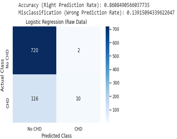
Confusion Matrix - logistic regression:#
results_lr = confusion_matrix(y_test, predict_logreg) print(results_lr) ax=sns.heatmap(results_lr,linewidths=1,vmax=1000,
square=True, cmap="Blues",annot=True)
#if i don't run the next 2 lines of code, the heatmap will be cut off. bottom, top = ax.get_ylim()
ax.set_ylim(bottom + 0.5, top - 0.5)

Although this post only take logistic regression as an example, but other models were also being tested. Here are the results:
models = pd.DataFrame({
'Model': ['Support Vector Machines', 'Logistic Regression','KNN',
              'Decision Tree','Naive Bayes', 'Random Forest',
              ],
    'Score': [SVM_score, Logistic_regression_score,knn_score, decision_tree_score, NB_score,
              RandomForest_score],
    'Kfold score': [svc_KFoldScore,logreg_Kfoldscore,knn_Kfoldscore,DT_Kfoldscore, nb_Kfoldscore,
rf_Kfoldscore]}) models.sort_values(by='Score', ascending=False)
| Model | Score | Kfold score |
|---|---|---|
| Logistic Regression | 86.037736 | 85.353774 |
| Support Vector Machines | 85.000000 | 84.481132 |
| Naive Bayes | 84.716981 | 84.410377 |
| Random Forest | 83.867925 | 83.066038 |
| KNN | 81.415094 | 82.075472 |
| Decision Tree | 74.905660 | 75.683962 |
Conclusion#
The model testing presents different results based on the two approaches, feature selection and feature extraction. With feature selection, gender (Male), age, cigarette consumption per day (cigsPerDay), history of stroke (prevalentStroke), increased systolic blood pressure (sysBP), and high glucose level (glucose) are suggested to be prominent risk factors for CHD. With these features, the logistic regression gives the highest model accuracy of 85.97%.